How to Divide in Excel

You don’t have to be a business analyst or an accountant to appreciate the advantages of using Microsoft Excel. However, not all users know how to use this spreadsheet tool properly.

So, without further ado, here’s a comprehensive guide on how to divide in Excel.

What Is the Division Formula in Excel?

There is no division sign on your computer’s keyboard, as you may have already noticed. The virtual keyboard of smartphones also doesn’t have one. Instead, Microsoft Excel and other spreadsheet apps use the forward-slash (/) for the division function.

The division formula in Excel goes like this: A/B.

A is the dividend or the number to be divided. While B is the divisor or the number you are dividing by. The result of the formula is called the quotient.

Hence, if we are to express a real-life problem in Excel, such as dividing $ 1,500 for a five-day budget, it would look like: 1,500/5.

How to Divide Numbers in Excel

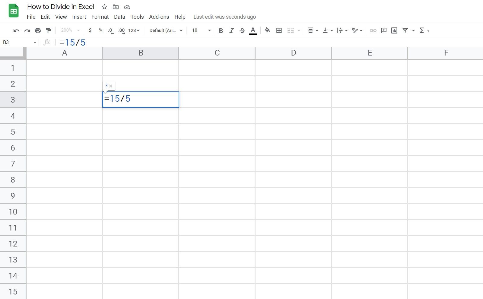
When creating an Excel formula, you must first type in the equals sign (=) into the cell where you want the result. Thus, if you wish the quotient to appear in a specific cell, here’s how you do it:

1. Click on the cell where you want the results to appear.
2. Type the equals sign (=), which signals to Excel that you’re generating a formula.
3. Type the dividend (the number to be divided), hit forward-slash (/), and then type in the divisor (the number to divide by). There shouldn’t be any spaces between these characters.
4. Hit Enter, and to generate the quotient in our cell.

How to Divide One Cell by Another in Excel

Suppose you have a table of data and want to use the existing cells as the dividend and divisor. How do you divide in Excel this way?

To do this, you need to understand that Excel designates alphabet letters for columns and numbers for rows to map out the spreadsheet table.

Click any cell in the spreadsheet, and if you look on the upper-left part of the Excel, just under the editing tools, it tells you the name of the cell. Hence, if it says G3, that means that the cell is under column G and lies in row 3.

Related: Crazy Excel Formulas That Do Amazing Things

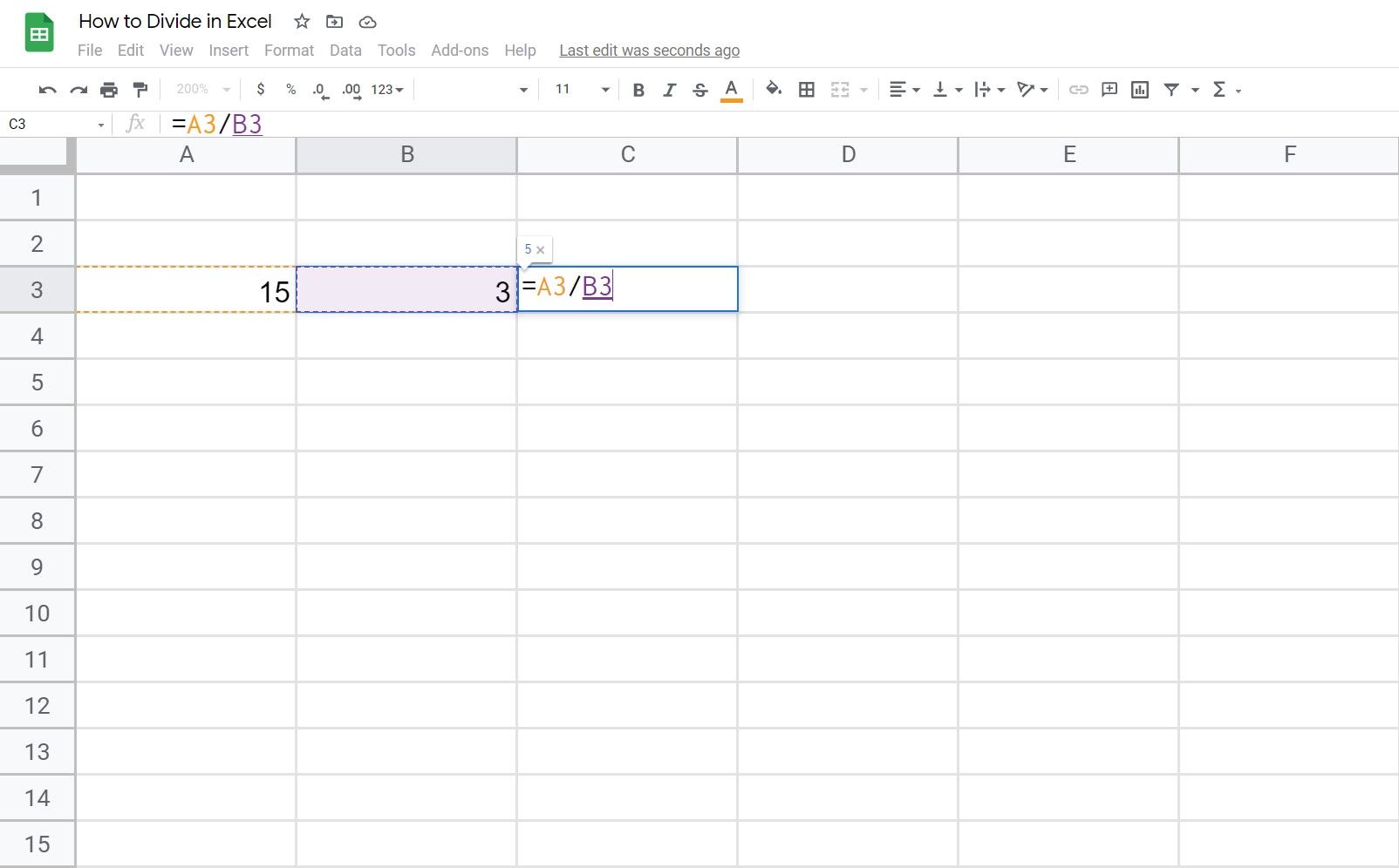
Let’s assume that cell A3 is your dividend and cell B3 is your divisor. You want to generate the quotient in cell C3. So, how do you divide in Excel this way?

Here’s what you should do:

1. Click on cell C3 and type the equals sign (=).
2. Next, move your pointer to your dividend cell (A3) and click it.
3. After which, hit forward-slash (/).
4. Then, click on the divisor cell (B3). At this point, you should have something like this: =A3/B3.

Finally, hit Enter, and it should display the answer.

If the values in your other cells change, the quotient in your results cell will update automatically.

Note that you can also type in a number to substitute your dividend or divisor instead of using a cell.

Thus, you can type in =A3/100 or 100/B3, provided that the cells A3 and B3 both have numbers in them.

Excel won’t process that formula if any of the cells have other types of data, such as text or images. Thus, you will likely encounter the error message #VALUE!.

How to Divide an Entire Column in Excel

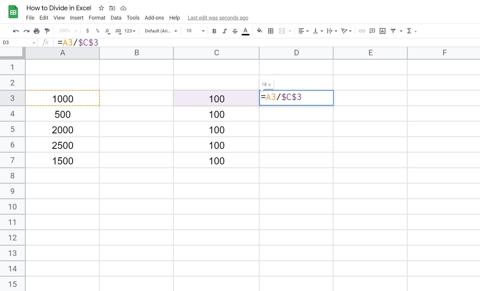
In some cases, you want to divide an entire column by a constant divisor, or vice versa. Let’s say you want to divide column A by a fixed number (say 100), which is in Cell C3. How do you do it?

First, you need to use a function called an absolute reference. By placing a dollar sign ($ ) in front of a column’s letter or a row’s number, you can lock in a specific cell as part of the formula. An absolute reference looks like this: $ A$ 1.

So here’s how to divide an entire column:

1. Select a cell in the column where you want the quotients or answers to be.
2. Type in the equals sign (=), then the first dividend entry, say A3. Follow it up by the forward-slash (/), then the absolute reference; in our case, $ C$ 3.
3. You should have something like this: =A3/$ C$ 3.
4. Hit Enter, and this should give you the answer.
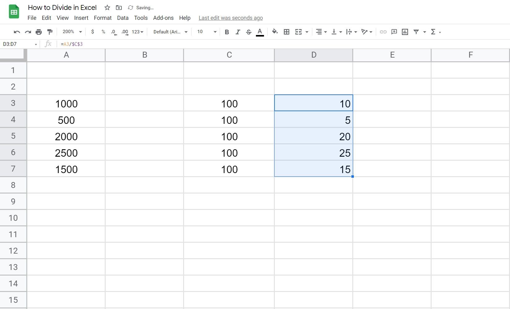
5. Next, drag down from the lower-right corner of the cell box. As you drag the pointer downwards it should copy the formula into the following cells.

In this case, cell C3 becomes the constant divider of the formula. Meanwhile, column A’s remaining cells are considered a relative reference and change from A4, to A5, and so on.

You can also use the Paste Special function without having to rely on using formulas. To do this, simply:

1. Click the cell of your divisor and then press CTRL + C (or Cmd + C on a Mac).
2. Select the range of your dividend, let’s say A3 to A7.
3. Right-click and then select the Paste Special option
4. Click Divide, then OK. It should give you the answers

Shortcut for Replicating a Division Formula

If you want to generate quotients for multiple target cells in one go, here is a shortcut

1. Click on the cell with a complete division formula, say C3. Make sure that the values in each row and column correspond to the correct divisors and dividends
2. Next, click on the lower-right edge of the box and drag the mouse pointer downwards or sidewards, depending on where you want the answers
3. After releasing the mouse pointer, it should display all the answers

If you ever see a #DIV/0 error, two things might have caused it. First, one of the cells involved doesn’t have any value in place or is blank. Second, the divisor cell has the number 0 in it. As you may already know, but dividing any number with zero results in an invalid equation

Exploring Other Division-Related Functions

Whether you are a student, a teacher, or a professional, learning how to divide in Excel is a valuable skill. Now you know how to divide in Excel, there are far more tasks you can use it for in your life.

MUO – Feed